Plots and reports

isaac_net.viz turns engine runs, benchmark results and the fidelity study's tables into figures in the paper's style, and RecorderLoop (isaac_net/core/record.py) records the per-step KPIs those figures need. Both live behind the optional viz extra. The core package imports neither matplotlib nor pandas.

pip install "isaac-net[viz]"          # matplotlib, pandas, pyarrow

Every image on this page comes from python docs/img/viz/make_gallery.py, which runs small seeded CPU jobs in about 30 seconds.

Record a run

from isaac_net import make_engine, record
from isaac_net.viz import cdf, report

net = record(make_engine("L2", E, R, dev, cfg), "runs/l2", every=10, label="L2 default")
for _ in range(T):
    net.submit(None, send)
    out = net.step(None, pos)              # the engine's own step dict, unchanged
net.close()                                # writes what is still buffered; `with record(...) as net:` also works
cdf.plot_delay_cdf(["runs/l2", "runs/l0"], by="level", path="delay.png")
report.from_records(["runs/l2", "runs/l0"], "report.html")

record(engine, out_dir, **kw) is RecorderLoop(engine, RecordConfig(out_dir=out_dir, **kw)). It wraps any engine from make_engine, including EdgeLoop, BackgroundLoop and EnergyLoop, in the same way EnergyLoop does. The engine API and the step dict stay the same. It is an explicit wrapper rather than an NRConfig field, so make_engine builds exactly what it built before. Wrap the outermost engine to see every key that the inner wrappers add (energy_*, bg_*).

The recorder does not change the run. It draws no random numbers and writes into no engine tensor, so every step output is bitwise the same as the bare engine's. tests/test_record.py checks this on L2 with multi-cell, background users, energy, RACH and DRX, and on L2-legacy and L0, with partial resets. Per step it only adds into fixed-shape device accumulators and makes no host sync (the test forbids item, tolist, cpu, numpy and the scalar conversions during the recorder's step). Every every steps it closes a window and stores one row per env in a device buffer of flush_every windows. Only a flush (buffer full, flush() or close()) copies data to the host and writes files. On a CPU, recording L2 with 64 envs of 16 robots adds about 3% to the step time.

RecordConfig field	Default	Meaning
out_dir	"records"	directory of the tables and meta.json
every	1	control steps per row
flush_every	256	windows kept on the device between host writes
format	"auto"	Parquet with pyarrow, else CSV; or "parquet", "csv"
per_cell	True	write the cells table
raw_envs	()	env ids whose robots get a row per window (robots table)
hist	True	write the delay and AoI histograms (exact CDFs to within one bin)
label	""	run name, a column of every table; by="config" groups runs by it
level	None	level name for the level column; None = the wrapped engine's level
tensorboard	None	log directory for torch.utils.tensorboard (needs the tensorboard package)
wandb	False	True logs to the active Weights & Biases run (one is started if none), or a dict of wandb.init arguments
log_every	1	scalar logging cadence in control steps

TensorBoard and W&B receive the env mean of delivered, lost, delay_mean_ms, delay_p50_ms, delay_p95_ms, aoi_p95_s, queue_bytes, prb_util, harq_bler and energy_j under net/, for every window whose end step is a multiple of log_every. They are written at flush time, so logging adds no sync either.

Tables

Each table is a directory of Parquet parts (out_dir/steps/part-00000.parquet, ...) or one CSV file (out_dir/steps.csv). isaac_net.core.record.read_records(out_dir, table) reads either as a pandas DataFrame, and meta.json holds the schema version (isaac-net-record/1), sizes, the control step length, the configuration summary and the column lists. Every table ends with the constant columns label and level. A column that the engine does not produce is NaN, so the schema is the same on every level.

Table	One row per	Columns
steps	window and env	step (control steps since the recorder was created, at the window end), env, episode (resets of the env since recording began), t (env clock), steps (window length); sums over the window: sent (accepted messages), offered_bytes, delivered, delivered_bytes, lost (timed out or dropped), harq_tx, harq_retx, energy_j; delay_mean_ms, delay_p50_ms, delay_p95_ms over the messages delivered in the window; aoi_mean_s, aoi_p95_s; window means of queue_bytes, queue_len, sinr_mean_db, access_idle / access_rach / access_connected / access_dormant (robot shares), los_frac, blocked_frac, bg_util; prb_util and dl_prb_util (PRB-slots granted over available, L2); harq_bler (first transmission); battery_frac (at the window end)
cells	window, env and cell	robots served at the end, delivered, prb_util (the robots' PRB-slots in the cell over the cell's available PRB-slots, L2), bg_util, bg_n
robots	window, env in raw_envs and robot	x, y (when step gets poses), sinr_db, serving_cell, queue_bytes, queue_len, access_state, los, blocked, battery_frac, aoi_s at the end; delivered, lost, delay_mean_ms, energy_j over the window
delay_hist, aoi_hist	flush, env and non-empty bin	bin, lo_ms, hi_ms, count: log-spaced bins from 0.1 ms to 60 s, about 6% wide (the bins of the benchmark metrics)

Delay is capture to delivery, the engine's delay times the control step. Age of information is computed per robot as in the Isaac layer's NetModule: the newest delivered capture, with the state at reset counting as known. The env-level prb_util counts every UE the NR MAC schedules, background ghosts included, while the per-cell prb_util counts the robots only and bg_util gives the background share. The PRB, HARQ and per-cell counters come from the NR engine (level L2). The per-cell PRBs use the read-only slot tap that EnergyLoop also uses (core/slot_tap.py).

Gallery

Delay and AoI CDFs

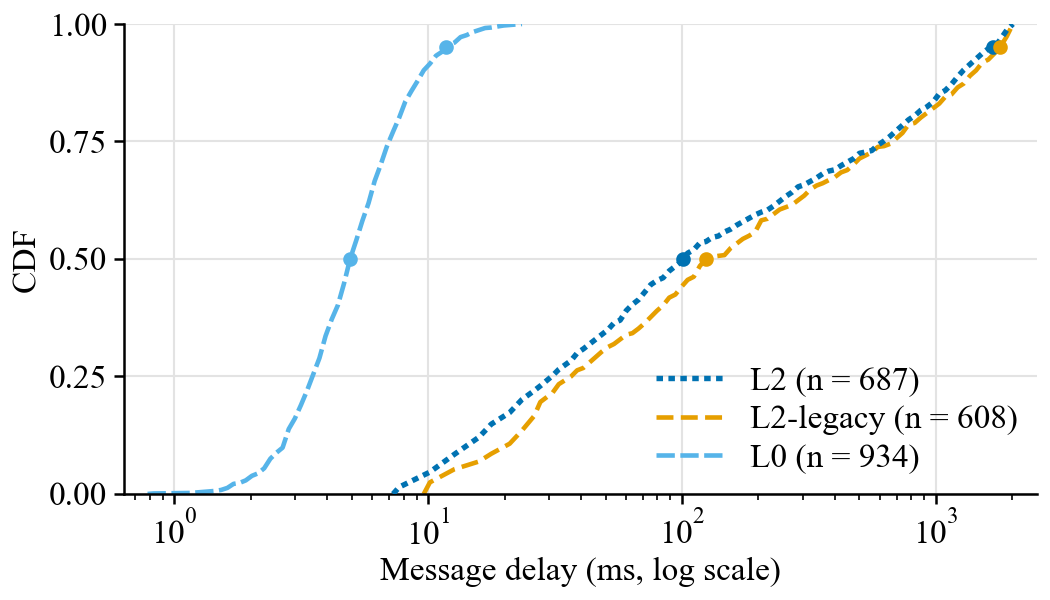
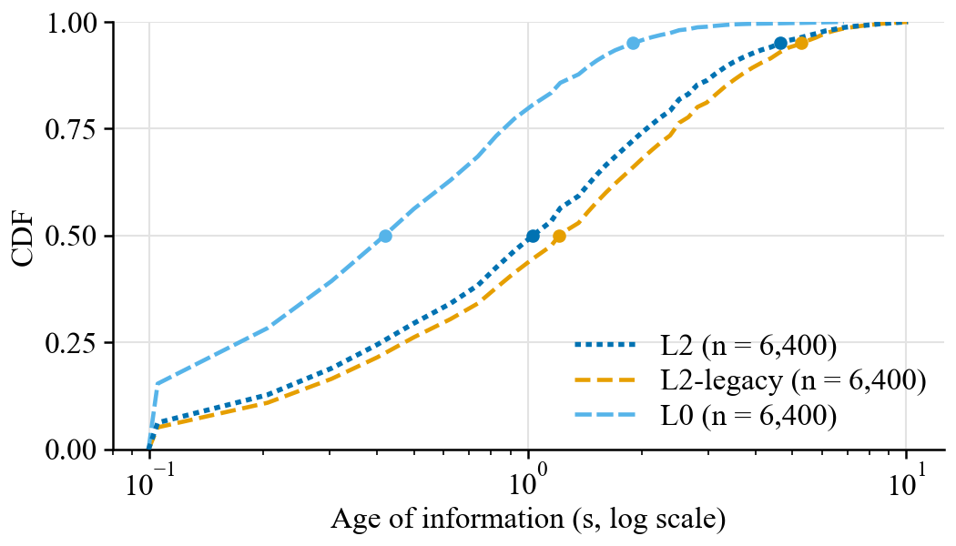
cdf.plot_delay_cdf(data, by="level") and cdf.plot_aoi_cdf(...) draw one curve per level (by="level") or per run label (by="config"), with dots at p50 and p95. The input can be recorder directories (their histograms give the CDF to within one bin), a frame table with a delay_ms column grouped by a column such as arm, or a dict of samples in ms. Below, the same random traffic runs on L2, L2-legacy and L0 (8 envs × 8 robots, 100 steps).

Throughput vs load

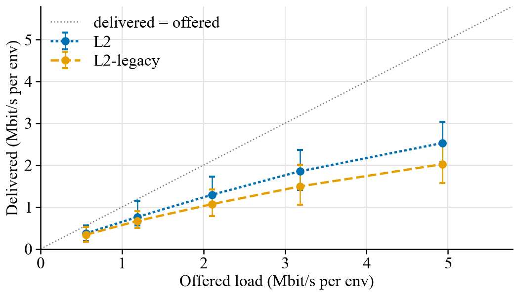
loads.plot_throughput_vs_load(data, by="level") plots the delivered against the offered rate per env. Recorder directories give one point per run (mean over envs, whiskers from the 10th to the 90th percentile over envs), so a sweep over loads traces a curve. Benchmark result directories and tables with offered_mbps and delivered_mbps columns work too.

Radio environment map

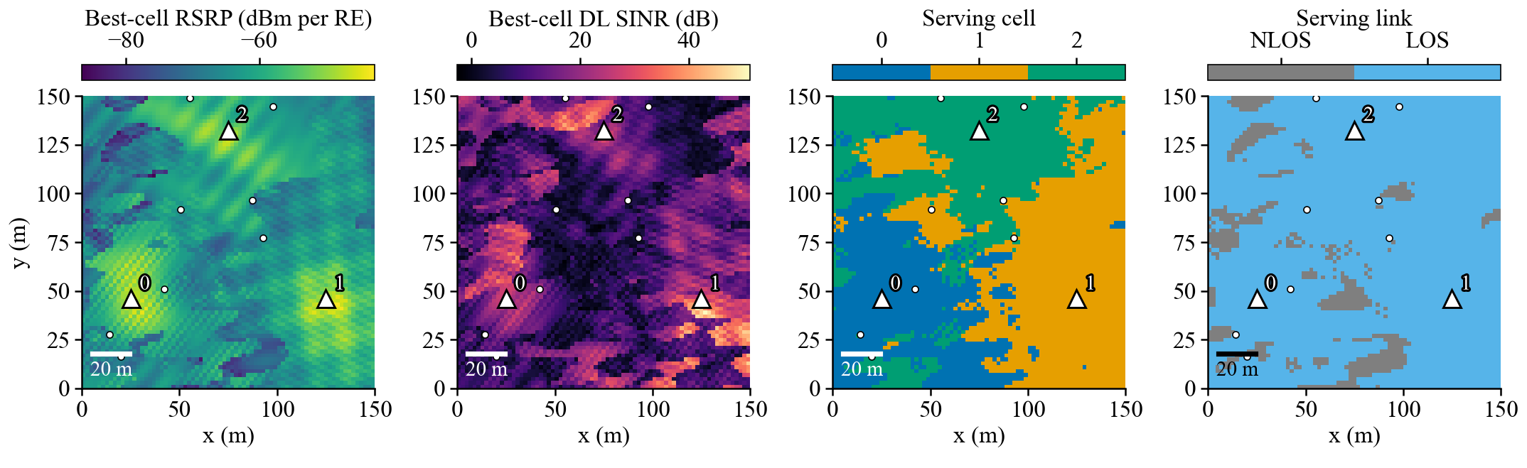
maps.plot_rem(rem, robots=None, panels=("rsrp", "sinr", "serving", "los")) takes the .npz file or dict from isaac_net.tools.rem and draws one panel per name, with the gNBs, an optional robot overlay and a scale bar. pathgain is also available, and los (the serving link's LOS state) needs a channel with a LOS state. isaac-net-rem --png rem.png --panels rsrp,sinr,serving,los uses the same function. Below are three cells with the TR 38.901 UMi channel at 2 m resolution.

Arena snapshot

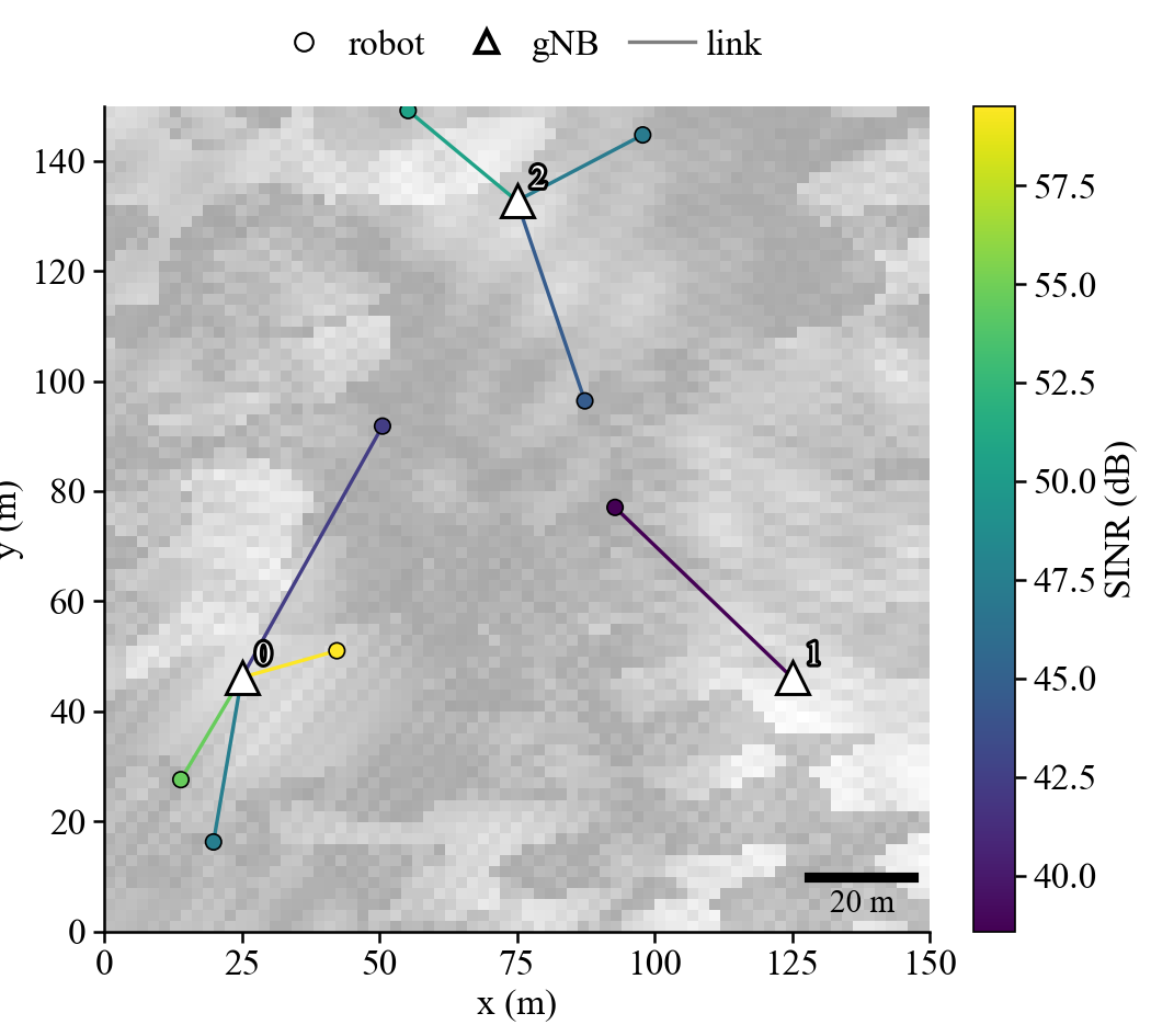
maps.plot_arena(positions, links, blocked, sinr, gnb) draws one env from above. Robots and their links to the serving gNB are coloured by SINR, blocked links are dashed, and a REM can be drawn faintly underneath (rem=). links takes the step dict's serving_cell, blocked takes out["blocked"] (the obstacle stack), and gnb takes positions or an NRConfig.

Per-cell PRB utilization

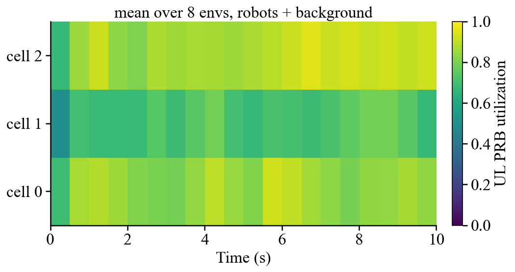
loads.plot_cell_utilization(record_dir) draws a cells × time heatmap from the cells table, either the mean over envs or one env (env=). The robots' and the background users' shares are added unless include_background=False. The run below has three cells with three background users per cell, recorded every five steps.

Engine vs ns-3 5G-LENA

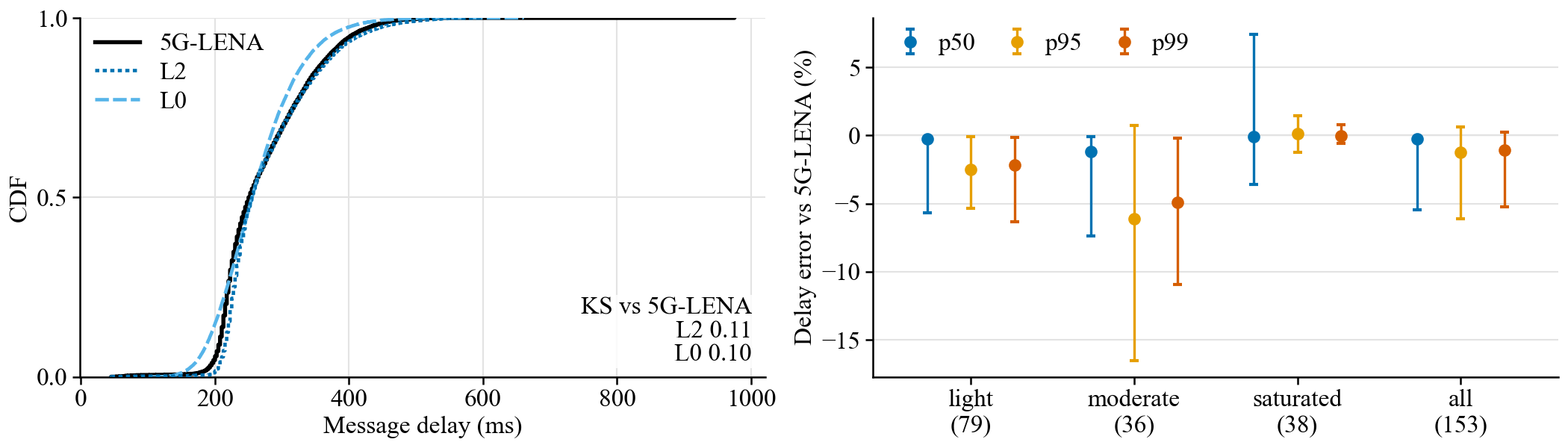
compare.plot_vs_ns3(engine_csv, lena_csv=None, per_run_csv=...) overlays the engine's delay CDF on 5G-LENA's and prints the KS distance of each arm. Frame tables have a delay_ms column, and one table with an arm column (such as benchmarks/results/closedloop/frames.csv.gz) is split into the ns-3 arm and the engine arms. A per-run table of the fidelity study (benchmarks/fidelity/results/*/per_run_<arm>.csv) adds the per-run errors of p50, p95 and p99: the median by load regime and over all runs, with whiskers from the 25th to the 75th percentile. Below, the left panel is the closed-loop run of closed-loop.md and the right panel is lena_validation_v2() over the 153 runs of fidelity-vs-lena.md.

Reports

• isaac_net.viz.report.from_records(dirs, "report.html") writes a self-contained HTML page with inline PNGs. It contains a summary row per run (delivered messages per env-second, loss, delay p50 and p95, AoI p95, PRB utilization, BLER, energy), the delay and AoI CDFs, throughput, and every run's per-cell heatmap. dirs can be a list of recorder directories or one parent directory.
• isaac-net-bench report results/ --html report.html adds the same kind of page to the benchmark suite: the Markdown table as HTML, the task metric of every configuration (mean ± 95% CI), a per-configuration table, and CDFs of the per-episode delay p95 and mean AoI per baseline for every task configuration. --figures DIR writes these figures as PNGs and lists them under the Markdown table. The CDFs run over the evaluation env-episodes when the result files keep their rows (isaac-net-bench run --keep_rows), and over the seeds otherwise.

Style

style.use_paper_style() applies the rcParams of the paper's figures globally: Times (falling back to STIX), 8 pt text, thin axes and no top or right spines. Every plot function also applies them locally (style.paper_style()), so package plots match the paper without changing the caller's settings. Colours follow the paper: L2 blue, L2-legacy orange, L1 purple, L0 sky blue, ns-3 5G-LENA black and Isaac Lab physics green, with the other Okabe-Ito colours for any other group (style.color_for, style.styles_for). style.COL_W and style.TEXT_W are the IEEE column and text widths. Every function returns its Axes (an array for multi-panel figures), saves the figure when path= is given, and accepts ax= (or axes=) to draw into an existing figure.